

Here is where we round things up and add a little to the explanation of the Perceptron and to look ahead to the next level of Machine learning:
In the Perceptron Introduction I posted this picture of the Perceptron with Bias:
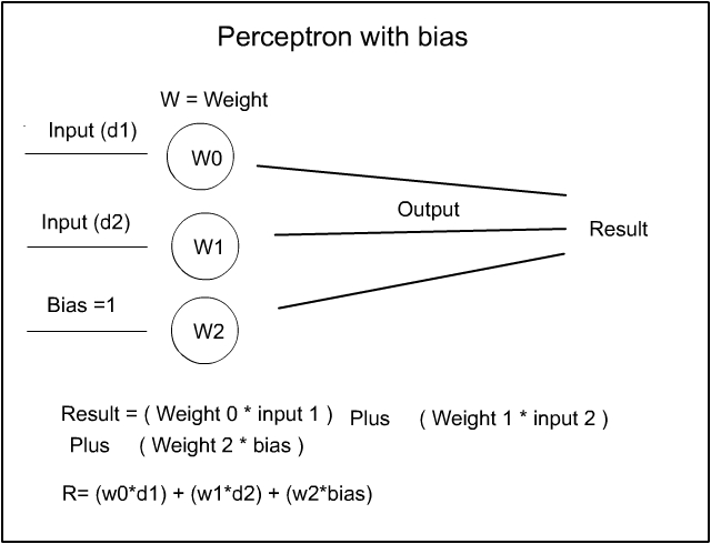
Many of you, who know a thing or two about the Perceptron diagram, may point out that ‘ I have left a little bit off the diagram at the ‘Result’ end ‘. Yes I did but that was intentional – I wanted to go through the math – especially the section on linear regression, bit by bit before introducing the whole Perceptron diagram – Here then, is ‘The Big Tomale ‘ :-
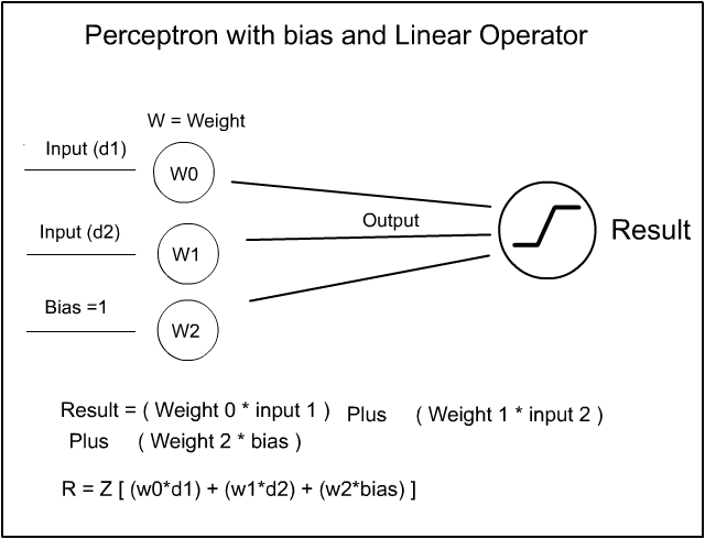
So the strange looking backward ‘ Z ‘ symbol is the symbolic function sign for Linear Regression. Now, as we have already covered Linear Regression in the Math section, where the output from the Perceptron is operated on through the Linear Function and the Linear result of that output is the new Result.
In which case, now you can now look at the full Perceptron diagram and see the output goes through the Linear function without the need for me to explain it all ! This avoids the complications of trying to explain the weird symbol right from the start. Because now, you already know what it is…
Others amongst you who know even more may say; ‘But that’s not the symbol I am used to seeing in the Perceptron diagrams’ – and, you are correct – the symbol you are seeking is the Sigmoid function : this one:-
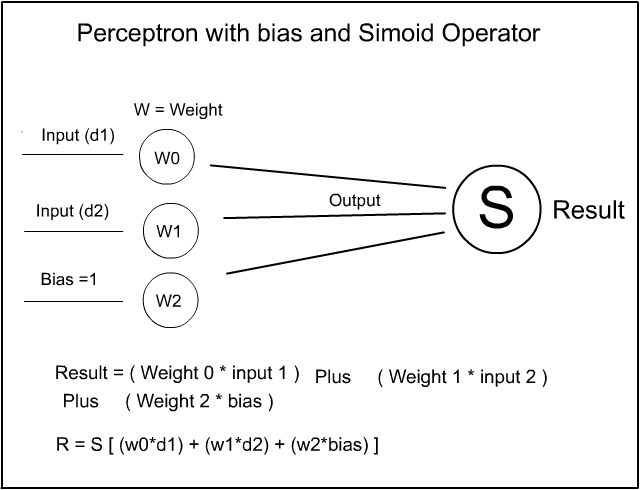
Yes that one !
The Sigmoid operator is in fact the Simple Logistic Regression function and works in much the same way as the Linear regression – except it is much smoother. However the Perceptron example we are looking at is suitable for using with Linear Regression. Don’t worry Logistic regression is just as simple and uses almost all the same basic techniques as the linear version.
Now I am mentioning this because many of the functions of more advanced Machine Learning use the Sigmoid Logical Regression operator so I need to introduce it here and now. Just to get used to it. So, this is what the Logistic Regression curve looks like :
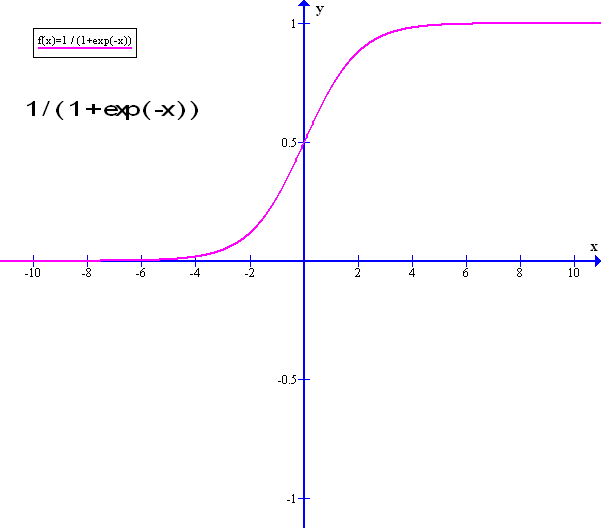
As you can see, the Logistic curve is nice and smooth – The X horizontal values go from zero to infinity and the Y vertical values are held between zero and one. So any number on the X axis will read as a value of between zero and one on the Y axis – smoothly. However the function itself is a little painful to look at and , as you can see, the formula is:
1 / ( 1 + e (-x)) – where ‘ e ‘ i is Eulers’ exponent. – see, not so friendly to look at
However, worry not, the function can be manipulated in much the same way as the Simple Linear function and as usual, the computer handles most of the Math – this is all but background information…
Simple Logistic Regression.
Going Back to our original example on simple Linear Regression – we have the following situation:
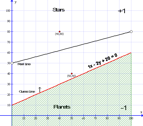
If you recall the red guess line was ‘ randomly ‘ set using the Gradient Formula of y = mx + c which, in this case was, y = 0.5x + 10 and the Standard equation ( ax+by+c=0 ) was 1x -2y + 20 = 0 ( as Illustrated above ) then we used the gradient formula to calculate the Error Factor which is the difference between the line and the data point at (50,40) towards which we wish to move. The Data Point illustrated is at (50,40) where x=50 and y=40 then we used the Linear Method to move the line.
Logistic regression is very similar to linear regression however, we do not need to calculate the error factor -in other words, we do not need to know how far a given data point is above or below the line – all we need to know is two things – is the given data point above the line or is the point below the line – that is all we need to know – the ‘Logistical Method’ then takes care of the rest…. To do this we simply need to use our ‘Standard’ formula ( ax + by + c = 0 ) rather than use the ‘Gradient formula’ ( y = mx =c ) directly in the math.
In the graphic above we see the guess line in Red is below the Data point (50,40) which would be labeled as -1 in our results table however our guess line is showing it is above the guess line and so labeled as +1 ( which is incorrect ). So we will need to move the red line upwards and closer to the Data point :
Now, WE can see the data point is clearly below the median line and that same data point is clearly showing above the red ‘guess line’ – this is all good for us but .. how does the computer know this? This is quite easy: The formula for the guess line is 1x-2y+20=0 – it important to notice that this formula equals zero. This means that every point on the line also equals zero – you can check this by looking at the point (20,20) which lies on the line – so plugging in the values into our formula : 1x-2y+20=0 becomes (1*20) – (2*20) +20 = 0 – this can also be seen at point (60,40) this too equals zero – so this is a neat math way of finding whether a point is on the line or not. ( if you want to miss out on the working out here – you can go straight to the Blue Box ‘Summary’ below…)
To find out how to do this take a quick look at the graphs below – all looks good – yes . The graph on the left uses the standard formula 2x+3y-6=0. The one on the right uses 2x-3y-6=0. Both graphs have a point indicated at point (5,4) – the graph on the right is a mirror image of the one on the left – And both points are above each respective lines..
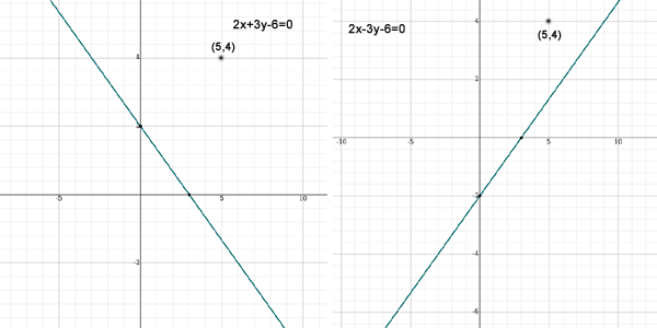
Now following the Logistic Method that I found on the internet – I was told, to find out if a point is above the line simply ‘input the data point values into the equation‘ and ‘if the result is positive the point is above the line‘ Really !! We shall see… – First we shall take the graph on the left – the equation is 2x+3y-6=0 and the point is (5,4) where x=5 and y=4 and noting that the Gradient is Negative – the line falls from left to right.. : So plugging away : ( 2*5 ) + ( 3*4 ) – 6 is equal to + 16 and 16 is positive and above zero and so is above the line – great. That’s all we need to do – Not so… Now let us do the same with the graph on the right : the equation is 2x-3y-6=0. The point is still at ( 5,4) and noting that the gradient is Positive – the line rises from left to right. So plugging the numbers in we get ( 2*5 ) – (3*4) -6 = – 8 and minus 8 is below zero and so according to the logic above – the point should be below the line – but of course it’s not is it – something else obviously needs to be done.
Looking closer it appears that – IF the gradient is Negative AND the result of the plugged in data point gives a POSITIVE result then the point is above the line. This is good – However IF the Gradient is Positive and the result of the plugged in data point is NEGATIVE – then the point should be below the line but it is actually above the line. Confusing – not really because, fortunately, there is a pattern forming – we are getting somewhere. So how do we tell whether a line has positive or negative gradient from the Standard formula?
Easy – Assuming that the ‘ax’ value is always set to positive then simply look at the ‘by’ value – it is the ‘by’ value alone that determines the gradient structure. for instance Graph 1 on the left has a formula 2x+3y-6=0 – Here the ‘by’ value is positive (+3y). Then the graph has a Negative gradient. Now looking at the graph on the right – the formula is : 2x-3y-6=0 – Here the ‘by’ Value is negative (-3y) – which means the graph has a Positive gradient. The gradient structure is formed by the sign of the ‘by’ value alone
Now we have a complete plan – looking to the graph on the left – Input the data point x and input the data point y ( 5,4 ) – Plug both of the numbers into the formula and see the result which is POSITIVE ( +16 ) – now check the gradient – as the ‘by’ value is POSITIVE ( +3y ) and as the RESULT is POSITIVE then the point is ABOVE the line – else if the result was negative the point is below the line –
Next look at the graph on the right – input the data point ( 5,4 )- plug in the numbers into the formula and see the result which is NEGATIVE ( -8 )- then check the gradient – as the ‘by’ value is NEGATIVE ( -3y ) and the RESULT is NEGATIVE then the Data point is ABOVE the line – else if the result was positive then the point is below the line.
In Summary – IF the sign of the result is the same as the sign of the ‘by’ value, the point is above the line – if the sign of the result is opposite to the sign of the ‘by’ value the point is below the line EASY = That’s it…
Now we can go back to where we were:-
So now, if we plug in the values of the data point at ( 50,40) we get this result: 1*50 – 2 * 40 +20 = -10 and -10 is LESS than zero and is NEGATIVE HOWEVER because our line has a Positive gradient – which means the ‘by’ Value is NEGATIVE (-2y) Therefore – the Result (being Negative) and the ‘by value (being Negative) means both are negative and the point is above the line – or rather the line is simply below the point.
If there was a data point ( not illustrated ) at say (50,20) which is below the guess line and again, plugging in the values ( 1*50 – 2*20 +20 = 30 ) the result is greater than zero and Positive – and looking at our ‘by’ value which is Negative (-2y) Which means, the result being POSITIVE and the ‘by’ value being NEGATIVE are opposite and therefore -the point is is below the line – In this way, we can test whether a point is above or below the guess line – without using the gradient error factor.
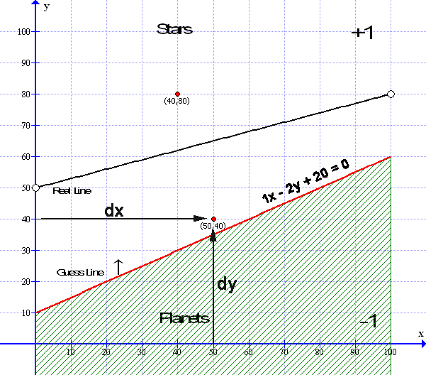
So in the above example – our guess line at 1x-2y+20=0 is below the ( 50,40 ) data point so the line needs to be tilted slightly and moved upwards. We can do this with the Simple Logistic Regression method shown below . All we need to remember is: if the data point is above the guess line we need to add to the guess line to move it up. And if the data point is below the guess line we need to subtract to move it down.
In the diagram I have indicated the point at ( 50,40 ) with a description o dx and dy – dx is simply the x value of the point and dy is the y value – however if you look at the Perceptron diagram at the top – I have used d1 as an input of data 1 and d2 as an input of data 2 – Here I am labeling d1 as dx for data x and d2 is labeled as dy for data y – Remembering that input data d3 is the bias and – our learning constant rate is 0.001. Now I can show you the formula used in the Logistical Method coming below:
The formula using ax+by+c =0 is : ( if the point is above the guess line then add: )
( a+ dx * learning rate ) x + ( b + dy * learning rate ) y + (c + learning rate ) = new guess line.
if the point is below the guess line then subtract:
( a – dx * learning rate ) x + ( b – dy * learning rate ) y + (c – learning rate ) = new guess line.
Simple Logistic Regression – the Method:
So using Simple Logistic regression using the standard equation of the line which is 1x – 2y+ 20 = 0. Looking at the lower data point at (50,40) is above the guess line we need to move the line upwards – which means we need to add all the factors – . To achieve this we take the x value of the data point which is labeled here as dx which is 50 – we multiply that number by the learning constant of 0.001 which is 50*0.001 = 0.05 this number is then added to the ‘a’ value of the standard line form so ‘a’ now equals 1 + 0.05 = 1.05. We do exactly the same with the y value – in this case labeled as dy, taking the y point at 40 multiplying by the learning constant 0.001 which becomes 40 * 0.001 =0.04 this is added to the ‘b’ value of the standard line – so the ‘b’ value of the line now becomes – 2 + 0.04 = -1.96. We then take the Constant C which is + 20 and simply add the learning constant to it – so C now becomes 20.001 and the final formula becomes 1.05x-1.96y+20.001=0. This formula can then be put directly into the weighs so W ( 0 ) = 1.05 w(1) = -1.96 and w(2) = 20.001. The Logic regression is then repeated until all the data points around the guess line all agree with the known data. And that is it!!
Now, I cannot currently show you a working model of a Perceptron using this Logistic Method as the code used in the Perceptron we have been looking at was set up to use the Linear Model – the only way to do this would be to reprogram the code which can be done but it will take time – I will get Bishop to look at it ( fat chance !! ). However you can check the above formula at www.symbolab.com and if you input the new line 1.05x – 1.96y + 20.001=0 and compare it against the original of 1x-2y+20=0 you will see the line has tilted and moved upwards but only very, very slightly so, Logistic Regression looks to be a lot slower than Linear regression. However, I do find that the Logistic Method to be more aesthetically pleasing than the Linear model.
There is much more to Logistic Regression than I have outlined here. Logistic Regression involves Calculus and Gradient descent , Maxima and Minima and derivatives – So apart from the above example, Logistic Regression is far beyond what we need for the examples I am using now but, from what I have seen, we will be bumping into again quite soon ! Oh dear….
Gradient Descent – A very Brief Overview.
Right I said on the last page we would be looking at Gradient Descent as it forms much of the basics of machine learning. We went through a similar method to the Logistic Regression above in our exploration of Linear Regression ( In the Yellow Box ) and we left it with this image and explanation :
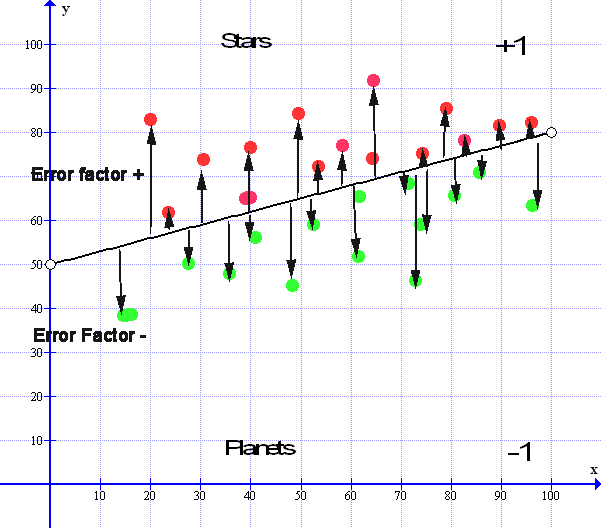
Now looking at the Median line we see that there are all the arrows pointing up, these are the upward error factors so they are all plus values. Then we see all the error factor pointing down, these are all the negative error factors – All of these error factors must balance out for the Median line to be at its optimum value:
So let us take all the Values of the Error Factors above the line and add them all together. We get a number that is say 257.0852. Now we take all the Values of Error factors that are below the line and add all those together we get a number that is – 257.0851. If we subtract one from the other we get a result that is = 0.0001 and if this number keeps constant between + or – 0.0001 then we cannot get any better than this and the median line is as good as we can get, especially with real life data and we can stop there. In effect, we are simply trying to get all the error arrows to reach towards a zero point :
However we can do a little more with these arrows. If we take all the arrows and place them in order of magnitude along a horizontal line with all the negative arrows on the left of the zero point and all the positive arrows to the right of the zero point you will find they all fit under a curve – like so
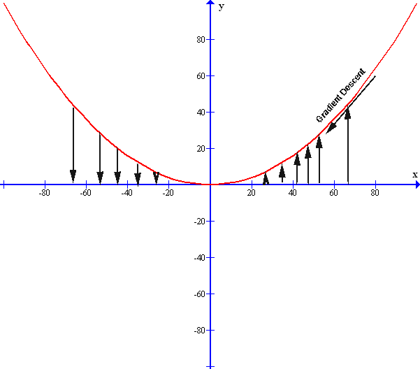
So, what we are doing with our ‘Linear Regression method’ in the previous yellow box – The ‘Method’ is to define a way of getting all the error factors to move towards the zero part of the curve by finding the derivative of the tangent at the point where the y point of the error factor touches the curve – However, this is far and way beyond what we need just now – this is just an introduction – The method outlined in the yellow box in the Linear Regression section is a simple, practical method to produce the gradient descent result – thankfully, without the need for any calculus – the same is to be said for the Logistic Regression method – it is practical without using calculus… Phew.
[ However there are ‘Machine Heads’ out there who ‘Program in Python’ and use ‘Pure Calculus’ for this Simple Regression – It looks good, sounds good but, we like simple here .. ]
If you would like a look at what Logistic Regression looks like then look no further than the Wikipedia article so Click Here for, as Bishop so eloquently put’s it – another Big Fat Fart in a Spacesuit.
This Concludes our look at the Perceptron – yes, this is it – Next we will look at how we can use these ideas to link many Perceptron’s – all linked together in a multi- layered spellbinding structure in the next enthralling episode of Neural Networking and the Quest for Machine Intelligence yay !!
Acknowledgments
- The Perceptron Linear Method – by Luis Serrano – his book can be found here https://www.manning.com/books/grokking-machine-learning
- The Perceptron Logistic Method – by Luis Serrano – his book can be found here https://www.manning.com/books/grokking-machine-learning
- Graph images compiled by ‘Graph’ courtesy of Ivan Johansen
- Other Graphic images by Lizzie Gray