

Right .. Now we are going to look at how the Perceptron works. To enable us to do this we can run the program, as before, by tapping on the panel below. It is the same program and code as our original example. This time however, there is a slope or gradient to the line – This is done simply to illustrate that the Perceptron can find a line of any gradient – the algorithm that runs the Perceptron is all the same code as before. So Click on the panel below, then, we can go through the workings…. Also there will be a link at the end where you can copy the program and play with it yourself.. Or if you just can’t wait you can just Click Here
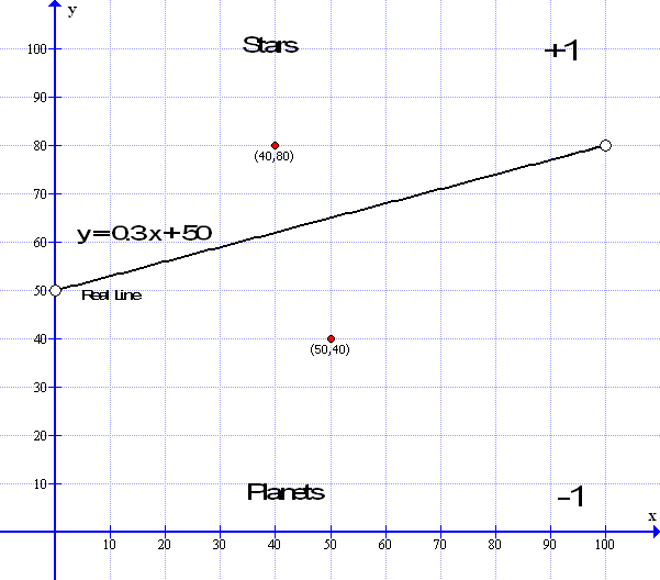
So what is happening here? The computer creates a space on the screen – in this case called a canvas upon which to draw its data. It draws the ‘data dividing’ line in white across the screen. In this case we are using a 3 in 10 gradient so, plugging the number into our straight line formula y = mx + c: the multiplier M = 3/10 or 0.3 in decimal and the constant C is at 50 as in our original example: so the formula becomes y=0.3x+50 ( However, because we are using a ‘mapping function’ in the code – the constant C is actually 0.1 but that is just a detail of the code )
While this all happens we can assign a small non zero random number to the weights in our ‘guess line’. The numbers typically look like this: Weight – W0 = 0.0172653 : W1 = 0.8872291 and W2 = 0.5198737
Weight W0 keeps track of the x coordinate of the guess line W1 is the y coordinate and W2 is the bias – or the C component – the height above the horizontal of the line – as I said in the original example – Bias is always set at 1 so Weight W2 is kept as it is ( 1 * w2 = w2 )
While all this goes on we can assign some random points for our data: In this case we will use 400 data points – you can have any amount of data but more points means a slower example to watch on the screen – less data points looses accuracy. 400 is not too bad. We can put all these data points into a table format; in computer speak this is called an array. In this way we can print out the same data points on each loop. At the same time we can test each point and attribute a +1 if it is above the white line ( A Star ) and a -1 if it is below ( A Planet ).
To do the next bit we will be using both the straight line ‘Gradient’ formula y=mx+c and the ‘Standard’ formula ax+by=c : Both are just variants of the same formula. I will add a diagram so it is easier to follow:
Now to assign whether a star is above the gradient line and assign it a +1 or whether it is below the line and assign it a -1 :
I have highlighted the next bit in blue as it is the method we use in the following learning process.
We can do this by using our formula y = mx + c: e.g. y = 0.3 x + 50 – So if say, data point 1 is at x=40 and y=80 – putting in the x values = 0.3 * 40 + 50 which equals 0.3 * 40 = 12 plus 50 = 62. We see that our y point is at 80 which is higher than the line ( when x=50 the line is at 62 ) so that data point is above the line and is labeled as +1 – A star. Conversely a data point at x=50 and y=40 – putting in the x values = 0.3*50+50 =65 and y at 40 means it is below the line at 65 so it is a planet and labeled as -1 ( See the diagrams above and below..)
Now we have all our data points in a table ( other wise called an Array ) – together with our correct answers +1 or -1. So we have everything together to be able to ‘teach’ our Perceptron.
To enable us to teach the Perceptron we use a ‘learning constant’. This constant is just a number – it can be any number; 1 or 0.1 or 0.001 or 0.0001. Now the larger this number, the quicker the Perceptron learns but the more inaccurate it becomes and the smaller the number the slower the learning process but the accuracy is improved – so its best to choose a number that is small but not too small as for the learning to take too long. In the case above we are using a learning constant of 0.001.
The learning constant is the number that we use to adjust the weights up or down to make the Perceptron’s ‘guessed line’ ( in Red ) come closer to the actual line ( in white ).
The program then draws in the red guessed line – I will come to this in a while – as, there is, in fact, no need to draw the red line each time but, it is drawn on each loop to demonstrate the learning progress in action – in fact the line need only be drawn at the end of the learning process ( epoch ) – however that would not be very interesting. So in it goes.
Now the algorithm goes through a long looping process. It takes each point in turn and compares that point against the guessed line in exactly the same process as in the blue box above. So if data point number one. Is a star or value +1 and the y value of the guessed line is also +1 then the answer is correct so we so nothing but move to the next point. If however the data point is -1 and the guess line sees it as +1 then we need to move the weights a little by adjusting the weights through the ‘learning’ constant. Then it repeats the process until all points are correctly allocated.
So how is this done? Before that, let us look at it logically first:
- If the Guess line reports a data point is +1 but the real answer should be -1 then we need to adjust the weights up by increasing them by the learning rate.
- If the guess line reports a data point is -1 but the real answer should be +1 then we need to adjust the weights down by decreasing then by the learning rate.
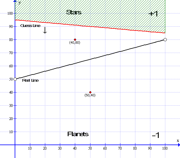
Here are the two situations: First we have the situation where the guess line reports a point at (40,80) is below the guess as -1 but the real answer should be +1 so the weights must be adjusted downwards by the learning constant.
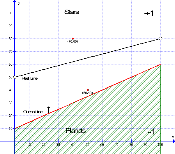
Next we see the guess line reports that the point at (50,40) is above the guess so it appears as +1 but it should be -1 so the weights must be adjusted upwards by the learning constant.
Now we get to the nitty gritty; We have to generate our guess line based on the random weights – to do this we use the ‘Standard’ straight line formula ax+by+c=0 where a and b are non-zero integer numbers that relate to the gradient M – where M = a / b So the formula ax+bx+c=-0 : Weight w0 =a , w1=b and w2 =c So the values of the Standard formula in wieghted terms becomes: – (w0)* x + (w1) * y + (w2) * bias = 0
Now, just in case you are not familiar about converting from gradient form to standard form here’s how it goes – In the diagram above – the red guess line has a gradient of y= 0.5x + 10 – you can see the y intercept when x=0 y is +10 i.e. when x=0 y=10 – To convert this to standard format first make the decimal part of the gradient 0.5 into a fraction which is 1/2 so the formula reads y = 1 / 2 x + 10 – now we get rid of the fraction by multiplying both sides by the lower part of the fraction – the 2 – so it becomes 2y = 1 x +20: moving the x to the left ( as in the Standard format ) it becomes -1x +2y = 20: then moving the constant C to the left we have -1x + 2y -20=0. Then getting rid of the untidy -x we multiply all of it by -1 which gets us to ( -1x + 2y – 20 = 0 ) * -1 which equals 1x -2y +20 =0 Tarah!
So our standard equation for ax+bx+c=0 : a and b becomes 1x-2y+20=0 which is also the same as 1x – 2y= -20 : You can check by saying what is x when y=0 ( cover up the y value with your finger ) and find that 1x=-20 and what is y when x=0 (cover up the x value) and -2y = -20 or y=-20/-2 = 10. So in this case, ax+by+c=0 : a=1 b=2 and c=20 – So weight w0=1 and w1=-2 and w2=-20. And as the gradient m = a / b : As in the above example gradient M = 1/2 or M=0.5 therefore the gradient M in our weighted example equals w0 / w1 : w0=1, w1=2 so w0 / w1 equals 1 / 2. Which fortunately, it does. And weight w2 is the bias which is equivalent to C which is 20.
Again this is a generalized view mainly to get the idea – the computer takes care of the math – however – if you want to see how the program handles it – it is like this:
x1 = xmin;
y1 = (-weights[2] – weights[0] * x1) / weights[1];
x2 = xmax;
y2 = (-weights[2] – weights[0] * x2) / weights[1];
line(x1, y1, x2, y2);
In the above example x1=min would be 0 and x2=max would be 100 and you can check it is correct by putting the numbers into the weight values e.g. (-20-1*0/-2=10 and -20-1*100/-2=-120/-2=60) so line drawn from x=0 y=10 to x=100 y=60. As can be seen on the red line in the diagram.
So now we can draw the guess line and from that guess line we can now test each data point to see if it is +1 or -1 we do this using the formula and method in the blue box above and, if the answer is wrong – we can adjust the weights a little – But How?
We can see from the diagram below that the lower data point at x=50 y=40 that is should be showing a TRUE result of -1 – however the Perceptron’s guess line shows it as +1 – which is WRONG and, as we saw before, the line needs to be moved upwards.
To do this we will use a tried and tested method used widely in statistics called by the ‘math speak’ name of Simple Linear regression – and in our case Very simple regression – worry not – it uses exactly the same formula as we know and love – namely the gradient equation above.
Simple Linear Regression
For now we will look at a general example and then bring it back to our Perceptron later. Say for instance, you have a spread of data points – very much like our Stars and Planets above. Now let us assume that all the points have some quality in common such as say the relative sizes of Stars and Planets- Now what we want to do with this spread of data points is find a line that fits all the points equally i.e the best fit ; Here is an example:
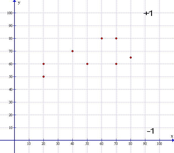
Here is a line that best fits the spread of data: So all the points are pretty evenly distributed above and below the median line.
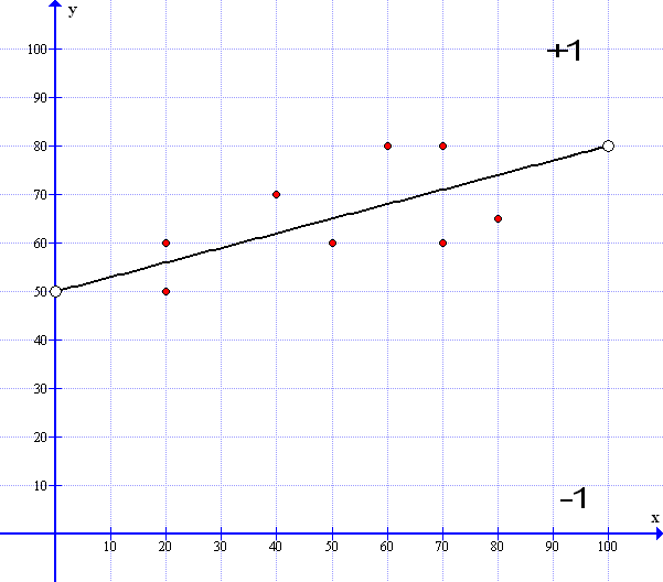
In effect – all the points above the median line are in the +1 domain and all those below the line are in the -1 domain – Looks familiar…So how do we get this median line? Well we start with a random guess line drawn in Red : Surprise!
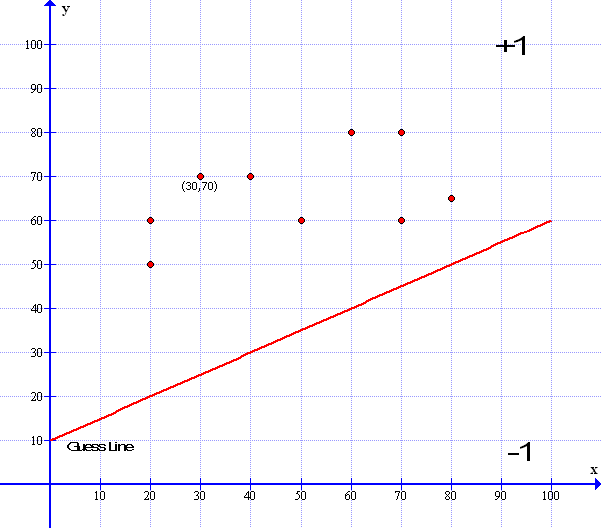
Now if we imagine that all the data points are like little magnets pulling the line up and down to fit – we could take each point in turn and just add a little here and a little there to make the line go up or down we could eve use our learning constant of 0.001 to add to the line- However sometimes we need to move the line down as well as up so we need to subtract the constant and not add it so how do we do this? This is where our favorite linear formula comes in. Now I have used the same guess line as in our perceptron example and the gradient formula for the red line is : y= 0.5x + 10 . Don’t worry too much about the red line formula as the computer works all that out for us.
Now we need to find a method – an algorithm that will give us the answer to how far away a data point is from the guess line so then we can see how much we need to move the line…
We saw earlier in our Blue Boxed section above we can test whether any data point is above or below the guess line by using the gradient formula y=0.5x+10. In the example above I have marked a data point at (30,70) so when x=30 y=70. We can see that it is above our red line. So what we need to do is lift the red line a little and change the slope to match the median black line we saw earlier. To do this we take the x value of that point (30) and plug it into our formula y= 0.5x + 10 : y=0.5*30+10 = 25 ( You can even see it is 25 by looking at the graph ). Then we can subtract the difference between the red line and the data point at y=70 which is 70-25 = 45. In effect the point is 45 units away from the red line. We can call this number ‘the error factor’ – Now to keep in line with our Perceptron diagram on page 1 – we had the inputs data 1 ( d1 ) and data 2 ( d2 ) So we can now label the X value as data x or dx and the error factor as data y or dy – And d3 – data 3 is our bias which we will deal with below. This now explains our data inputs. Continuing…
So looking at our formula ( y = mx + c ) y = 0.5x + 10 – By examining the chart above – we can see that we need to lift the red line upwards and adjust the slope to fit towards the median ( Black Line ) we saw earlier. And here is the method that achieves this:
In Math speak this looks like M = M + ( error factor * dx * learning rate ) and
C = C + ( error factor * l earning rate) —
Or as in the above m = m + ( dy * dx * learning rate) and c = c + ( dy * learning rate)
Now to explain:
Looking at the method in detail we have the following situation –
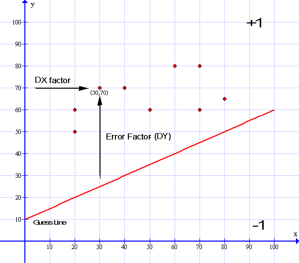
Linear Regression Method (Gradient Descent)
First, we take the error factor – dy of 45 together with the x distance – here called dx Factor- of the point at 30. We multiply the dx factor distance (30) by the dy error factor (45) – which equals 1350 – We then multiply this result by our learning factor of 0.001 – this becomes 30 * 45 * 0.001 = 1.35. We then add this value to our gradient so the gradient now becomes 0.5 + 1.35 = 1.85. – Now we also need to move the bias constant C up to meet the median line -this we do by multiplying the dy error factor (45) by the constant C (10) which = 450 then we multiply this by the learning rate 0.001 – which = 0.045 which we add to C so C now becomes 10.045 – And the whole formula now becomes y = 1.85x + 10.045 – we see the Guess line has moved up a little and the gradient slope has tilted upwards towards the point – the slope will eventually even out towards the median line as it nears the other data points.
This method takes care of all of the upward and downward movements of the line as any points below the line will result in a downward movement as the error factor will be negative and, as we get closer to the median line, the error factor will get less and less until all the errors are minimized. .. Thus all is taken care of – all we need do now is convert the formula to the standard form of ax+bx+c=0 to draw our new line. And, put all our new numbers into the weighted values.
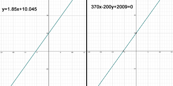
Now previously – I gave an easy example of y = 0.5 x + 10 which can be standardized easily giving the standard equation 1x – 2y + 20 = 0 ( See the Yellow Boxed Section above ) In which case Weight w0 = 1 w1= -2 and w3 =20 – Here we now have a big problem as we have to make the new equation into the form of ax+by+c=0 to input into the weights – where a, b and c need to be whole integer numbers. And, as you can see, the gradient M = 1.85 and the constant C = 10.045 – not very integer whole numbers .. Fortunately we have help – here in the form of a website that does this all for us. The website is www.symbolab.com – you can find it if you Click Here – So if you put in the formula y=1.85X+10.045 – ‘symbolab’ does all the working out for you. and reveals that a= 370 b= -200 and c=2009 – However for those with a hearty stomach – I will take you through all the steps below:
So, our new formula for y=1.85x+10.045 needs to be reformatted a bit and we find that as a fraction 1.85 = 37/20 so the equation now becomes y=37/20x +10.045 : multiplying both sides by 20 it becomes 20y=37x+200.9 Now we neet to make C a whole number integer which we do by multiplying everything by 10 so the formua now equals 200y=370x+2009 finally 370x-200y+2009=0 :- Therefore a=370 b= -200 and c= 2009 In which case w0=370 w1= – 200 and w2= 2009. Phew! I know its O.K. because I drew the graph to check! Like so-
Now you see why it is best to leave the computer to take care of the maths!
So finally: in conclusion – Looking back at our Perceptron graphic:
From the point of view of our red guess line – the ‘Planet’ at data point (50,40) should read -1 but is in fact reading from the guess lines point of view as +1 in which case we need to calculate the error factor and use the linear regression method to move the line upwards just as we did in the example above. Then repeat and repeat and repeat again and, that is as good as it gets! – well Sort of….
Now ( just because I am a Secret Sadist ) – we are not just going to leave it there – oh no. The question remains – How do you really know that our little Perceptron’s Red guess line really fits the median black line? Well that is straightforward:- If you imagine that all the data points above the median line are like magnets pulling the line upwards – and all the data points below the median line, like magnets, are pulling the line down wards then it is only when the pull upwards equals the pull down wards that we find the exact median line – but, how can we do this? Our points are not magnets they are just points of numerical data…
This is easy – just take all of the Error Factors above the line – add them all together – then take all the Error Factors below the line and add them all together – then we subtract one from the other and, if it equals or, is close to zero then that is it – if it all equals out – we are all done – let us look at this in a little more detail – ( you will see why soon – there is a little more to Machine Learning, which we need to know for later. It called Gradient Descent. However I will come back to this in our Conclusion on the next page.. )
Here is a small graphic that illustrates this:
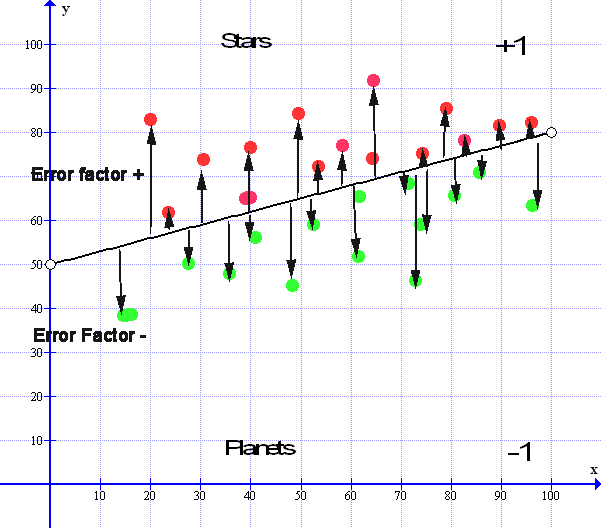
Now looking at the Median line we see that there are all the arrows pointing up, these are the upward error factors so they are all plus values. Then we see all the error factor pointing down, these are all the negative error factors – All of these error factors must balance out for the Median line to be at its optimum value:
So let us take all the Values of the Error Factors above the line and add them all together. We get a number that is say 257.0852. Now we take all the Values of Error factors that are below the line and add all those together we get a number that is – 257.0851. If we subtract one from the other we get a result that is = 0.0001 and if this number keeps constant between + 0.0001 or – 0.0001 then we cannot get any better than this and the median line is as good as we can get, especially with real life data and so we can stop there.
So to end our Perceptron program we could just keep a tally of all the error factors above the line – then subtract these from all the error factors below the line and when they reach near zero – the gradient has descended – we are all done – program ends – line complete.
Then, when all is complete, and the guess line closely matches the real line – we can input a data point and ask the Perceptron ; ‘Is this a Star or a Planet?’ and the Perceptron will answer – ‘I’m Sorry Dave but I can’t do that…’ *
- Quote courtesy of Stanley Kubric’s film 2001 & Arthur C. Clarke
Sorry couldn’t resist the joke there no, when the learning session has been completed the computer can use the final ‘guess’ line together with the gradient ( or Standard ) formula to test whether any newly input Data point is above or below the line and will then report whether it is a Star or a Planet. Job done…
Now, for your delectation, you could look at the Wikipedia article on Linear Regression: Click Here but its rather awful to read … Bishop says reading the article is about as pleasurable as having a fart in a spacesuit.
By now we have all had enough so I will put the Conclusions that I was originally going to put at the end of this page into a new page called Perceptron3 – Conclusion. Here, we can round up all that we have looked at and draw our Perceptron diagram complete with the linear regression algorithm we have just looked at – From this we can expand this algorithm into another level which will lead us towards the next level of Machine Intelligence and from this to well .. I know, you just can’t wait……
However, For now, you can download the Perceptron program and have a good play about with it – you can change the data size, change the learning rate, change the slope of the graph and do lots of exciting things – So, for the Example page you can Click Here.
Or you can look at the Conclusion and Intro into the next phase of Machine Madness by clicking the next menu tab Perceptron 3 – The Conclusion or alternately you can just Click Here
Acknowledgments.
- P5JS Code based on text “Artificial Intelligence”, George Luger
- Original coding by Daniel Shiffman -The Nature of Code – http://natureofcode.com
- Additional coding by In Variant B – http://lizziegray.net
- Graph images compiled by ‘Graph’ courtesy of Ivan Johansen
- Additional Graphs and formula by www.symbolab.com