

Linear Algebra for Machine Learning – Basics
Hi and welcome to our little post on Linear Algebra – Here we will be looking at what Linear Algebra is and how it relates to Machine Leaning. Here we will be using all of the examples in our Machine Learning posts so that if you read this first then all of the examples in our Machine learning will be easily understood.
Now, all of these examples will be easy, in fact so mind- numbingly simple that most of you will be yawning – but don’t fret it does get more challenging later. Linear Algebra simply deals with straight lines – lines tilted up – lines tilted down and there is only one formula to understand in Linear Algebra l. Now there are those who say that linear algebra also deals in three dimensional planes – this is correct but, we don’t need that yet so, let us begin with the Basics:
The Number Line.
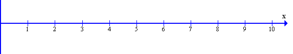
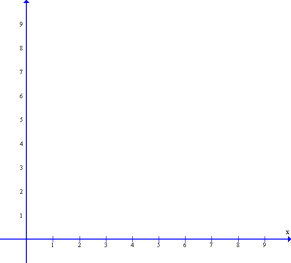
Take a line – any line and draw it horizontally from left to right. Then add in a few integer numbers such as 1,2,3,4,5 and so on:
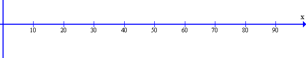
Or it could be – 10,20, 30, 40.
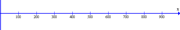
Or even – 100,200,300
Or perhaps even 1M,2M,3M…. and just keep on going – all the way to forever – to infinity and beyond.. So what do we have? This is the number line. A line that contains all the countable numbers that are possible to have. It is a lot of numbers…
Now take a look at the numbers between zero and one – now we can half this to 1/2 half it again to 1/4 and again to 1/8 and again 1/16 keep on halving until the fractions become infinitely small:-
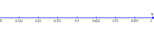
Keep on dividing – until the divisions of the number line go onto infinitely tiny infinitesimals . So here between zero and one there is yet another infinity of tiny divisions – Now take the number between 1 and 2 and do the same – yet another infinity of divisions – do the same between 2 and three and on to infinity .. So between every integer number from 0 to infinity there is an infinite number of divisions to infinity – so what is an infinite number of divisions taken to infinity – well that is just infinity. Infinity really is that big.
The Axis.
So now we have our horizontal number line – we can, just for fun, call this line ‘x’ why? Why not. Then we can draw a similar line vertically upwards. We can add the same numbers onto our vertical line as on the horizontal line – this line we can call ‘y’ Why? exactly… Anyway we now have two lines one horizontal called ‘x’ the other a vertical line called ‘y’ we can now call these lines Axis – so we have an ‘x’ axis and a ‘y’ axis with nice integer divisions on each.
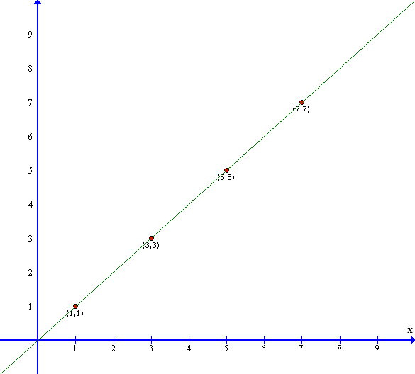
We can then draw a small dot onto any part of the page and we can trace an invisible line down to where the dot would cross the x axis and make a note of the number – we can do the same with the y axis and find the position of the dot to be ( x,y ) or ( 3,3 ) where x = 3 and y = 3 or x=5 and y=5 or even (7,7) where x=7 and y=7
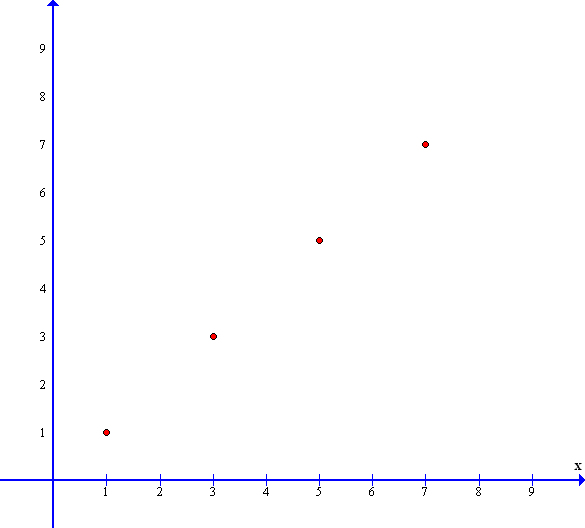
These numbers form the Cartesian co-ordinates of the dot – Cartesian named after Rene Descartes who published this method in 1637 . We can now plot other points on the graph and each point would have its own co-ordinate. This way we can locate the position of all the data points on the graph. We can also draw a line that joins through all these points and if this results in a straight line – we have a straight line graph…
This co-ordinate system provides us with a tool to be able to link geometry with algebra. Geometry – Algebra ? but, how? Let us find out:
Geometric Linear algebra
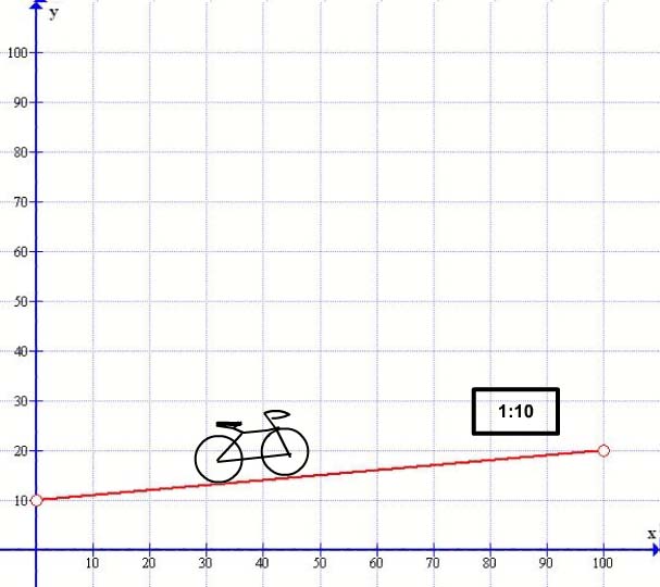
Say for instance you are riding a bicycle up a hill – a geometrical incline – and you are getting thoroughly puffed out. You wonder to yourself – ‘How steep is this ‘bleeping’ hill ?’ Let us look at it (from the side) in two dimensions flat:
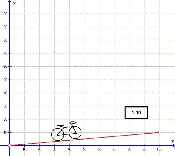
Here you will see our road in red, here drawn from the side on – you will see a horizontal line in blue – our ‘x axis’ which goes from zero – the starting point – up to 100 – an arbitrary end point. There is also another blue line our ‘y Axis’ that goes vertically from zero to 100. You will also see that our road in red rises from the left to right – this is known as a positive gradient. Now as you climb up the incline you see a sign before you : The sign says 1:10 – and you think what the heck does that mean? What this sign means is that the upward incline gradient is 1 in 10 ( no, not the current unemployment rate ) It means that for every 10 feet / yard / meter / mile / light-year that you go forward ( Horizontally ) you rise ( Vertically ) upwards by 1 foot / yard / meter / mile / light-year. So, for every measurement forwards you rise 1/10 of a measure upwards. This can be seen on the graph as, when the graph on the horizontal reads 100 the number on the vertical reads 10 – forwards 100 – rise 10 – the Gradient Slope is one in ten. So if the horizontal line went to 1000 then the red line would rise to 100 etc, etc, etc. on to infinity.
Now we can see the red line slopes upwards and if you look at where say x=100 you can see that the value on the y axis is 10 and also when x=50 you can see that the value on the y axis is 5. In other words the y value is simply the x value multiplied by 1/10 or y is equal to x/10. In other words each time x increases by one y increases by 1/10.
We can generalize this – if we call our gradient slope M then y=x*m where in this case m=1/10 the gradient being 1 in 10. And this is our first formula !!
The Gradient Formula : y = mx +c
In general terms the horizontal ‘x’ value is known as the independent variable and mainly increases in regular steps such as 1,2,3,4 or 10,20,30,40. Y is known as the dependent variable as the value of y depends on the slope of the line – at any value given by x. So, say for instance instead of 1 in 10 say the gradient M is 1 in 2 then y=1/2 x so every time x increases by one, y increases by 1/2. So our formula becomes y=1/2 x or y=0.5 x- . I like to call gradient ‘m’ the ‘multiplier’ because you have to multiply the gradient m value by the x value to get the y value. Hence y = m*x…
Here we have transposed a geometrical slope into an algebraic function – hence linear algebra.
Now let us look at a similar slope but raised up a little:
Here as we travel uphill on our bike we are on the same slope but it has been raised from the zero origin at x=0 to a point 10 units above the horizontal line. In our original slope when x was 100 y read as 10 – here when x = 100 y reads as 20 – the slope is the same it is just moved up 10 points – so every point moved by x you need to multiply the gradient 1/10 then add 10 to it each time. So looking at when x is 50 then y= 1/10*50 + 10 =15 which it is ! Now this lifting of the line gives us a constant which here is 10 and we give the constant a letter and this letter is C (Some use B instead but I like C for ‘constant’ better ) . So now our formula becomes y= mx + c or y = 1/10x + 10 – and this is it – this is the full gradient formula. We have done it, we have transposed a geometric gradient slope to an algebraic formula…
Now we have slogged our way up the hill but, what happens to our formula when we come down the hill – let’s see – going uphill where the slope increases from left to right is known as a positive gradient – going down hill where the slope falls from left to right is known as a negative gradient Like so:
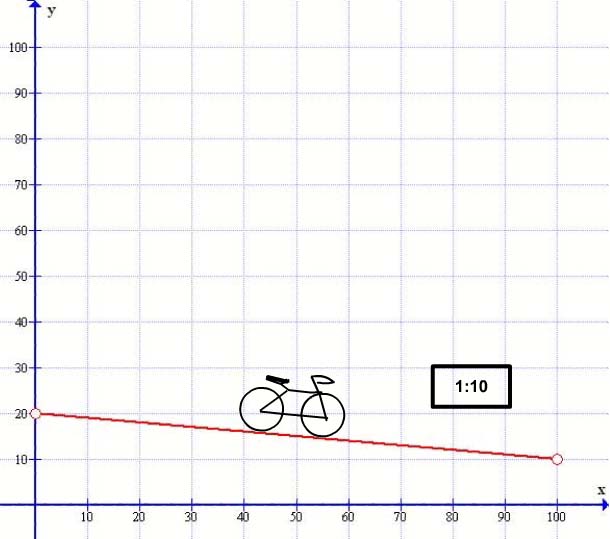
I have matched the gradient as 1 in 10 so the slope is the same but down wards and I have taken the start point where the last graph ended at 20 – This time the gradient is negative so the M value is minus M. So what does our formula look like now. Simple y = ( minus 1/10 x ) + 20 or y = – mx +c – Just to check when x= 100 y= ( -1/10 *100) +20 = 10 : which you can see by the graph it is. Similarly when x = 50 y= (-0.1*50) +20 = 15. O.K. (Note 1/10 as a fraction is the same as 0.1 as a decimal ) O.K.
Gradient Formula Plus .
So what can we do with this formula – Well, in machine learning sometimes we need to know how far a point is above or below the gradient line line so that our line can be moved to the correct level. Also in the graphic below I haven’t illustrated the gradient either so we need to calculate the formula first:
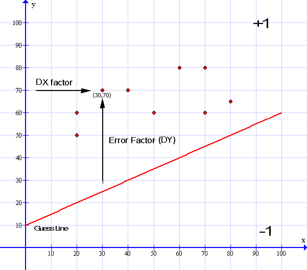
Now the red line cuts the y axis at 10 so we know that the ‘c’ value is 10. We can also see that when x is 100 y is equal to 60. So we need to find out what our gradient is in respect to x and y. Dropping the line down by 10 to reach the base line is subtracting 10 from 60 or in algebra terms is subtracting c from y – which is (60-10=) 50 so when x= 100 y now = 50 and dividing y/x to get the gradient y/x = 50/100 which is 0.5 or 1/2 so gradient m=1/2 – Using our formula y=mx+c we can rearrange the formula as above for m like this: m = ( y – c ) /x. Which is m= ( 60-10 )/100 = 1/2 so here m=1/2 or 0.5 in decimal and the gradient formula for the red line above is y = 1/2x + 10.
Next looking at the point at (30,70 ) where x =30 and y = 70 we can also see it is above the line but by how much? First we need to find the position of the line when x=30 as y is the dependent variable of the line – so taking the x value of that point [ labeled above as dx ] which = (30) and plug it into our formula y= 0.5x + 10 : y=0.5*30+10 = 25 ( You can even see it is 25 by looking at the graph ). Then we can subtract the difference between the red line y value and the data point at y=70 which is 70-25 = 45. In effect the point is 45 units above the red line.
Here, using our formula, we can see how far above the line our data point is. In machine learning we need to do this to enable us to use our ‘learning algorithm’ to process data correctly.
This is all we need at the moment with our gradient formula now we need to look at the same formula but this time in its Standard form.
The Standard Formula : ax + by +c = 0
At first glance the standard formula looks rather different to the gradient formula but it is exactly the same formula – just shuffled around a bit. The standard formula is ax+by + c=0 and can also be written as ax + by = c where a , b and c are all integer values. But what does it all mean? First let us look at the gradient graph using the same formula as in the example above : y= 1/2 x + 10
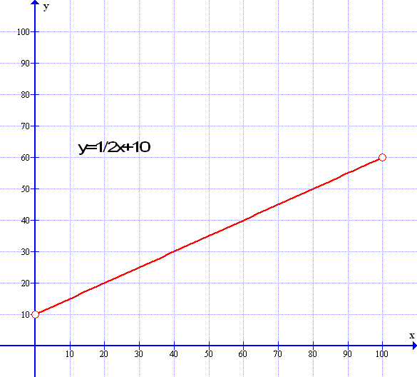
We can see that the gradient formula y = mx + c means that m is the gradient of the line – the rise in height over the horizontal distance – so in the example above y = 1/2x + 10 and the constant c is the intercept where the line cuts the y axis when x=0
To get to the standard formula take the gradient formula y = 1/2x +10 and get rid of the fraction 1/2 by multiplying both sides by 2 – the formula now becomes 2y = 1x + 20. Now move the x value to the left and it becomes -1x+2y=+20. Make the x value positive by multiplying everything be -1 and it becomes 1x-2y=-20. Then if you wish you can move the c value to the left and it becomes 1x -2y + 20 = 0 and, there we have it… in which case a=1 b=-2 and c=20 like so:
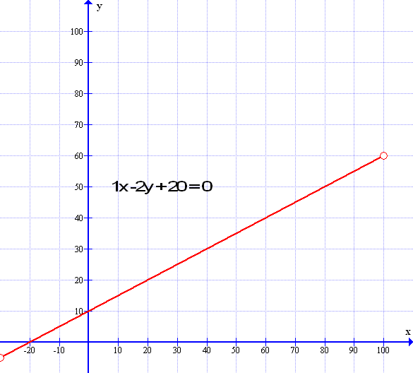
So its the same graph but why use the standard formula? Because it is a quick way of drawing a line – using 1x -2y = -20 when y is zero – by covering up the y value with your finger you will see that x = -20 and when x = zero cover up the x value with your finger and you get -2y=-20 or y= 10 – you can use those two values x=-20 and y=10 alone to draw the line. As you can see in the graph above the line cuts the y axis at +10 and it cuts the x axis at -20 : these two points then define the gradient slope of the line. Indeed – the gradient slope of the line can be defined as a / b = 1 / 2 = 0.5 and 10/20 = 1/2.
Also in machine learning we use ‘weighted’ values to calculate the new lines in the learning algorithm and the weighted values correspond to the ‘a’ the ‘b’ and the ‘c’ values of the standard formula. The gradient formula is used in the ‘error factor’ as described above.
Hence in Machine Learning, both formulas are used fairly equally and so it is useful to know how to manipulate them. However, it’s not too vital to know all of this in great detail as the computer does most ( all ) of the math and manipulations – this is just background knowledge for you to see what the machine is actually doing..
So that’s all we need to know about Linear Algebra for now – there is of course, lot’s more to Linear A and I will probably need to add to it as we go along but, this will do for now – So all you need to do is look over the Perceptron section and you will see all of the above formulas being used to great effect. So either click on the menu tab above for the Perceptron page – or alternately – you can just Click Here.
Acknowledgments:
- Graph images compiled by ‘Graph’ courtesy of Ivan Johansen
- All other Graphics – Lizzie Gray