

Multi Level Machine Learning
Here we are going to look at Multi Level Machines. A Multi Level Machine is simply a network comprised of a number of Perceptrons all linked together to make a Live Neural Network. In order to explain things as we go along there will be a real time example of a MLM Network running in real time at the end of the section. In this way, all of our explanations can be related to our real live example Network for you to play with.
In our previous sections, we looked at the Perceptron and noted that it has limitations. Limitations in that it deals with simple Linear functions – straight lines and definable blocks of Data. (Stars and Planets). Here we will look at situations where the data is more complex. Situations where Machine Learning is involved with non-linear data such as pictures and images – specifically image recognition.
As an example, let us take a look at the following image:
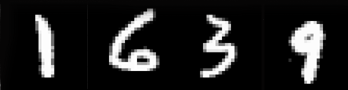
Hopefully you can read the number it is 1639 and is handwritten by several different people. ( It was also the year that the first printing press was set up in America. )
Now this is fairy easy for us to read but imagine writing a program that would be able to read just the following number:
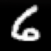
The program to do this would be horrendous, you would need to distinguish the space before and after the digit then look at the space inside the digit, you would need to find the the edges of the number then plough through many algorithms to tell which is background and which is the number. Then after finding the edges then you would need to figure out what the number might be. It would not be a good task to endure…
Fortunately we do not need to write a computer program to do this complex task – a Neural Network can do it all for us, in not too many lines of code.
Multi Level Neural Network.
Multi Level Machines can be called by many names: These can be Multi Level Machines (MLM). Multi Level Machine Learning (MLML). Neural Networks (NN). Associative Neural Networks (ANN) and Convolutional Neural Networks (CNN). Fortunately whatever they are called, they all boil down to the same thing – many Perceptrons all linked together – one Perceprton linked to all other Perceptrons through a Network of connections – All woven together just like a very simple tapestry.
Here is a reminder of our diagram of the Perceptron we saw earlier:
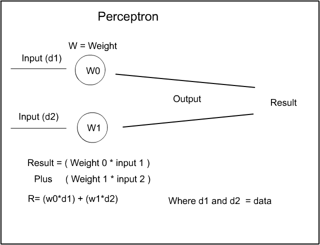
So now let us assume all we need do is simplify the diagram and link several Perceptrons together with several inputs and an output :-
Now, this would be perfect if this example worked, but, it doesn’t work. Early experimenters tried structures similar to this in the early days of Neural Networks and none worked. One simple reason for its failure is to realize that neural networks are built on structures that seek to model the workings of the brain and the network above can be likened to having the input data ( Sight ) coming into the eyes and so the result would only show the input of the eyes – with no subsequent understanding. This is not how the brain works – People saw that the optic nerve came from the eyes then the signals entered a convoluted mass of neurones, synapses and connections. It was this Neural Mass that was the key to enable the brain to understand what it was seeing – so the key is to add a convoluted layer of connections to the Perceptron input. As in the diagram below: Fortunately it was found that the following structure did, in fact, work.
The Neural Network.
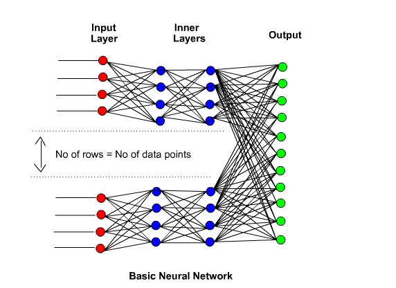
On the left hand side we see the input data stream – on the right hand side we see the output result. In the centre of the diagram we see the Inner Layers of the network. It is these Inner Layers that make the network Convolutional. The Perceptrons that accept the input data are all connected to the inner layers – each layer is connected to each other and the final layer is output to the Perceptron output – This makes a Convolutional Associative Neural Network.
[ The inner Layers are sometimes called the ‘Hidden Layer’ but this terminology is a bit ‘Geek Speak’ and hints at a little ‘ bogus mystery’ towards Neural Networks so we will not be using this terminology – However best to be aware of this common usage. ]
The structure of data:
So how would it be possible to input a picture of a numerical digit into a Neural Network – what kind of data does a picture contain that a Neural Network can understand ?
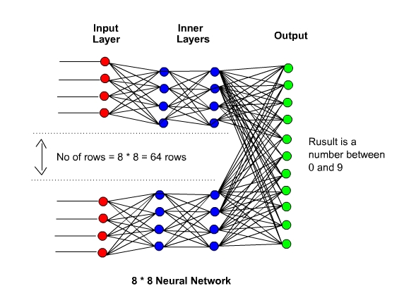
For our main example we will be using a Neural Net that analyses the numerical handwriting of the individual digits that we looked at in the first part above. It will do a training run where the handwritten digits are guessed initially, and checked against the correct result. If the answer is correct then do nothing otherwise all the Perceprons will be adjusted until the network gets them correct ( more right than wrong ). As soon as the training run is getting mostly correct results – ( this will be revealed by a correct percentage output reading ) – Then we can then input our own digit in our own handwriting and see it the network guesses our number correctly – The output of the Network will be a result which will be between zero to nine. Hopefully we will see if it guesses our number correctly.
So, in using pictures of numbers, we will look very briefly at how computers store and display both letters, numbers and pictures to the screen – the screen you are now looking at:
This is the number one: ‘ I ‘
In computer terms the number one is held in an 8 bit matrix array like so:
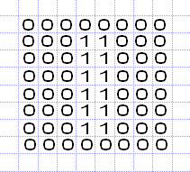
This is called a bitmap image. As you can see the top row consists of 8 zeros, the next row consists of a three zeros two 1’s and three zeros = 8 bits = 00011000. The next six rows are repeated and then 8 zeros at the bottom row. This makes and 8*8 matrix. Now, the computer screen consists of tiny cells called Pixels so that when the number 1 is put into the monitor screen, say at the top left of the screen. We program it so that the zeros do not show up and all you see is the number 1’s in the bitmap displaying in a vertical straight line in the corner of the screen denoting the number one. This is where the term bitmap image comes from – each bit ( 0 or 1 ) is mapped directly into the top eight by eight pixels onto the screen.
Now in modern screens there is a bit more to it than this simple example, such as colours and brightness Plus: black is actually zero (B 00000000 ) and white is 255 ( B 11111111 ) but, at the basic level this is all there is needed to know. Pictures all follow this pattern so any picture can be displayed onto the screen as a bit map of ones and zeros.
Here is a similar simplified example for the number two. However, this time we have reversed the image so that the background is 1 and the highlighted number 2 is zero: Just to keep in line with the current convention where zero is black:
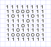
However, just but looking at this oversimplified example – here you can see that the bitmapped image would be and ideal source of data for our neural network. Starting at the top we have eight rows and eight columns = 64 unique numbers that contain the data that denotes the numbers from zero to nine.
So, all the numbers from zero to nine have a unique set of data points that denotes each number. This is this kind of data that we can use to input into our neural network. The output for our data will be the result of the network which will be a output of zero to nine:
So all we have to do is use the computers own data structures to input any image ( or Voice Audio / Music ) into the network to provide an output result. Now we can look at the data set we will be using on our live example and we can then walk through the process:
The MNIST data set.
Going forward with our live example Neural Network we are going to use images that are scanned copies of handwritten numbers. ( the same ones as in the example number at the top of the page ). These images come from the MNIST data set. The MNIST database of handwritten digits, has a training set of 60,000 examples, and a test set of 10,000 examples. You can view and download the whole data set by Clicking Here.
Each image of the data set is comprised of a hand written image that 28 * 28 bits in a grey scale image. Each bitmap pixel will contain a number between 0 and 255. Where 0 is black, 255 is white and 128 is a shade of grey. The MNIST data images are contained in a ubyte format which is a python format however we can convert ubyte with p5 javascript routine and you can see the images below: Click on the screen to get it running…
The data set comes in two parts – one is the image itself and the other is the correct result of the image ( Shown below the image in the viewer above ).. The image data can be input into the network and the output result can be checked against the correct answer.
You can look at the numbers as they scroll past, it will take a while but it is useful to look at because, when we go into our live example you can adjust your writing a little to match the script if your digits differ too much from the data set.
This ends the basic introduction to Multi Level Networks and you may wonder why we are using pictures of numbers to demonstrate Neural Networks. This is because the MNIST data set is a large available dataset to use for training and you can check the effectiveness of the network directly as you will be drawing your own numbers into the input box and the output result will be live.
Also this method is the root basic method used in all Neural Networks. Whether it is face recognition or voice recognition – It all uses the same method. Once you have learned this method that is it… Everything else is just more of the same. The networks may get bigger, wider or deeper but, in essence, it all boils down to what you are going to see next.
So look out for Multi Level Machines – The Learning …. coming next.
Acknowledgements
- You can find the p5js MNIST viewer code by Clicking Here
- ( Extra Coding by Variant B )
- MNIST data set – http://yann.lecun.com/exdb/mnist/
- All other graphics by Lizzie Gray : www.lizziegray.net