

The Perceptron – A Brief introduction.
During the 1950’s there was a BIG move forward in computing technology ( the invention of the transistor together with bigger storage capacity ). This came in conjunction with the development in the neurone theory of the brain ( above ). Both of these things led to the perceptron algorithm which was invented in 1958 at the Cornell Aeronautical Laboratory by Frank Rosenblatt. The first idea of an artificial neurone network – the artificial Perceptron .
The perceptron seeks to replicate the working of a neurone unit by either ‘firing’ ie conducting a current or not, as the case may be. The perceptron was originally constructed as a true machine using resistors and capacitors – The original machine tried to recognise facial features using a perceptron learning algorithm but due to the limitations of the machine and trying to ‘perceive’ a complex image using a simple neurone net, this simply did not work – So, due to the initial disappointment with the machine, the idea was eventually dropped.
However, interest in the idea of the perceptron continued and it was later found that if the perceptron was built into a multi- layered design using software rather than a machine, with many virtual perceptron’s linked together then, many of the initial limitations could be overcome.
For now, we are going to look at the perceptron as it is the cellular equivalent of a neural network. To do this we will delve straight into the perceptron algorithm.
Now, like I said in the Home Page, there is a little Math here but its quite simple and only involves basic high school adding and multiplying – the math is called Linear Algebra and its about straight lines. So if you can understand this :
y=mx+c or ax+by+c=0
Then carry on. If the formula looks goofy then look at the section called Linear Algebra – its really easy. This can be found under the Neural Network sub heading at the top menu – alternately you can Click Here.
The Perceptron.
So in order to create an artificial neurone – a perceptron – we need to replicate a neural unit – a brain cell – We know that the real neurone either fires or it doesn’t so, what we need to do is create a situation where the artificial neurone ‘fires’ at a certain point. What is done to achieve this is, that a ‘weight’ is assigned to the perceptron. The weight is nothing more than a number – a number that is assigned to that perceptron. Now the weight can be a small near zero random number. Initially the value of the weight is fairly unimportant as it will be adjusted over time. This adjustment is part of the ‘learning algorithm’ which will increase or decrease the weight until the perceptron gets the answer correct. If the perceptron gets the answer correct then nothing more is done. If the perceptron gets the answer wrong then the adjustment to the weight is continued until the perceptron gets the answer correct. We will look at this in more detail with the next example. For now, here is the usual diagram of a basic perceptron.
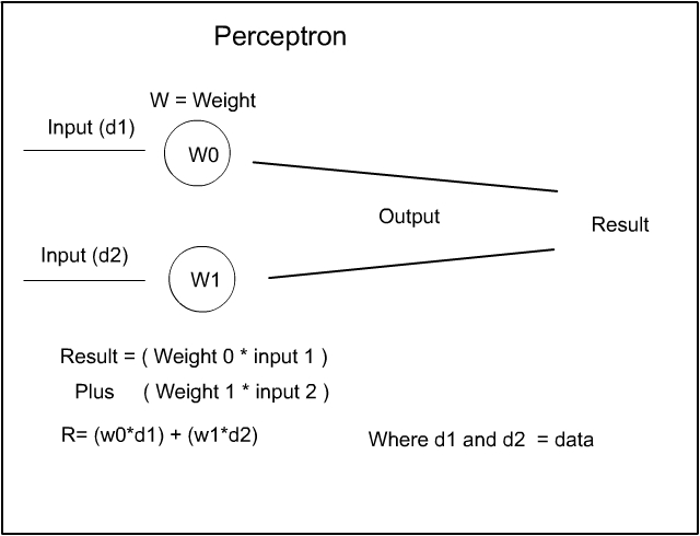
Here you can see that Data is input into the perceptron – we will get to ‘Data’ in a minute – the data (d1) is multiplied by the Weight (W0) and a result is out put. This is also added to any second bit of data (d2) this too is multiplied by the weight (W1) and the result is (w0*d1) + (w1*d2) – In effect – this is multiplying each weight with the input data and adding them together to produce a ‘result’. This is all we need for now to get the basic idea of what the perceptron is doing.
So, what are these ‘weights’ and how are they stored in, say a computer. Hopefully many of you know what a spreadsheet is. Spreadsheets have lines and columns in a table format that allow you to enter data into each cell and they allow you to use formulas such as multiplication and addition to produce a result. If so, then – could you produce a perceptron algorithm in a spreadsheet ? – yes you can, sort of – it would not be an efficient way to get a result and the graphics on a spreadsheet also lack the ability to display the result of the perceptrons’ output agreeably. However, computers do not need to use spreadsheets – they can hold data in their own table format – these are called arrays – sometimes called matrices. However, spreadsheets, matrices, arrays are all the same – just tables holding and manipulating numerical data.
Perceptron with Bias
Now, because the Perceptron works with Linear Algebra there is one more concept to discuss. Linear Algebra deals with lines and slopes – gradients. These linear graphs use the formula y=mx+c as shown below –
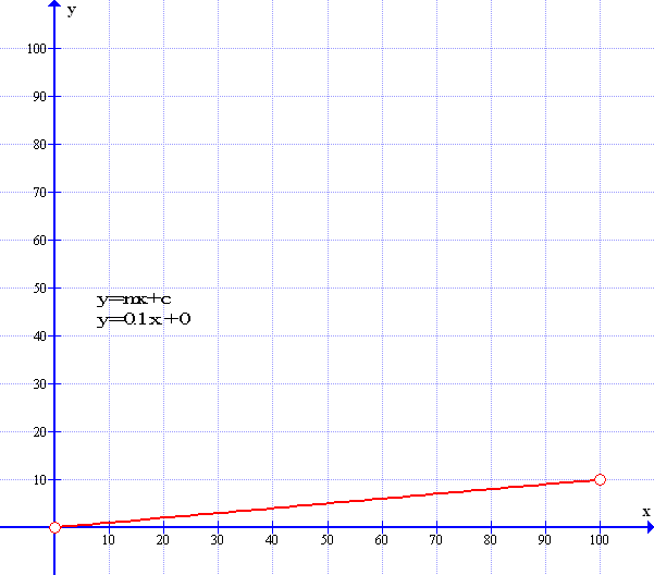
As can be seen the graph has a gradient of 1 in 10 where m=0.1 However the graph starts at the zero origin point. So that the constant ‘C’ is zero. The next graph starts where y=10 – it is moved up by ten points: The constant ‘C’ is now ten – So the formula now is y=mx+10.
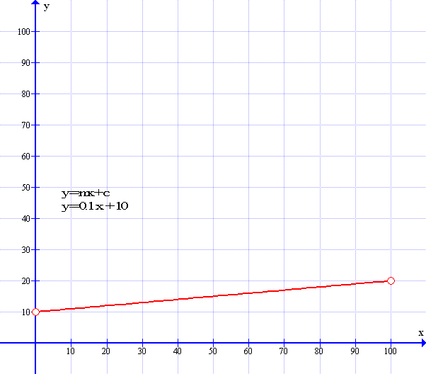
So if we understand that the weights (w1) and (w2) deal with the slope of the graph then we need a value to be able to slide the graph up from zero to 10 in this case – this is where Bias comes in – bias simply moves the graph upwards or sidewards to match the linear formula. In fact, we can re-write our graph formula of y=mx+c to y=mx+b – where b=bias. Bias, like weight – is just another number in a cell array and, in most cases, Bias is just set to one. So now we can see the next image of the perceptron this time with bias added.
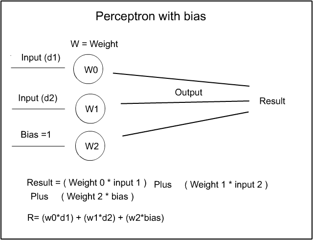
As before, the bias is simply multiplied by the weight and the result is added along with the previous result to produce an output result. Now, as the Bias is always one – then all we need to do is use w2 as it is because, anything multiplied by 1 is itself i.e 1*2 = 2 so w2*1=w2. Hopefully that is all Hunky Dory.
Now if you didn’t understand everything in the above don’t worry as this is just background information – I didn’t get it first time either… . The next example will explain what the perceptron is trying to do and later, how it does it too.
Perceptron – A Simple example
We are now going to look at a very simple example of the way a perceptron acts, what the weights and bias do, what data is and, the importance of accurate data. Now there are many forms of data that can be used in perceptrons – many examples use cats and dogs, circles and squares etc but we, at Bishops insistence will be using Stars and Planets !
Here in the graph Stars are above the line because they are large and Planets are below the line because they are smaller than stars – but some stars are small and some planets are large so there will be a good data spread but also allow for a clear line of difference:
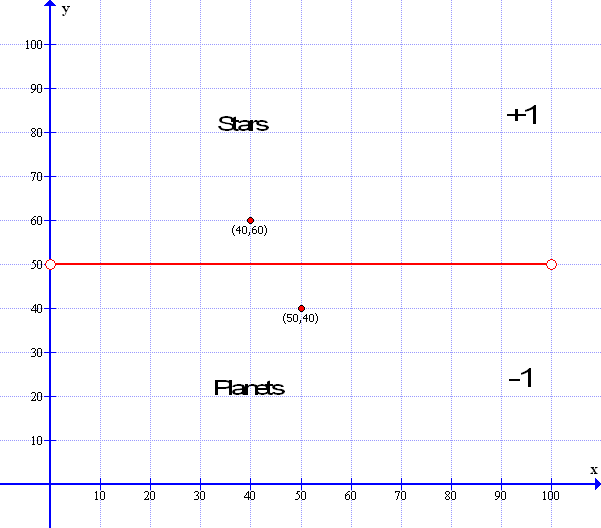
This is an illustrative graph set from x=0 to 100 and y=0 to 100. There is no gradient on the line so if y=mx+c then the gradient Multiplier – M=0 and constant – C in this case is set at 50. For ease, There are only two data points: a Planet at x=50: y=40 and a Star at x=40:y=60. So every data point below the line of y=50 is a Planet and everything above the line at 50 is a Star: To make it easy for the perceptron all points above the line ( Stars ) are labeled as +1 and all points below the line ( Planets ) are labeled as -1.
So all the perceptron has to do is match that all the data points labeled as +1 are above a line that we randomly create in the computer using the random weights – called the ‘guessed line ‘ and all those below are -1. However if the Percptron’s guessed line is at a wrong level then we use a ‘learning algorithm’ – a supervised learning strategy to raise or lower the line a little at a time until all the answers are correct.:
Firstly, we know what the actual line is – so we get the computer to mark all the points above the real line (Stars) as +1 and all those below (Planets) as -1. So now we know all the correct answers. Then we allocate a small but, non zero random number to each of the three weights – this allows the perceptron to draw a randomly guessed line – that may or most probably, not fit with the real line. Then we ask a question for each point on the guessed line:
If the point is above the guessed line it is then allocated a value of +1 A star. If the point is below the guessed line a planet – it is then allocates a value of -1.
Now, we know the real answer because, we just worked it all out in the sequence above if the point is above the guessed line ( +1 ) and the real answer is also ( +1) then that is correct so we do nothing. If the real answer is +1 and our guessed answer is -1 then we need to change the random weight a little – raise, or move the line a little at a time – until the answer becomes correct.
This is the ‘learning process’ more accurately a ‘guessing and moving process’ -this loops round and round and round and round until all the answers to the points on the guessed line match all the answers to the points on the real line then – if all the answers are correct then – Schools out and we finish.!!! FAB. Otherwise keep on looping.
Now, we are not tooo concerned if the guessed line does not exactly match the original line as in the example below the guessed line could fit at any angle or any point in the dotted area – all we are concerned about is that the answers are all correctly labeled as +1 – Stars and -1 Planets.
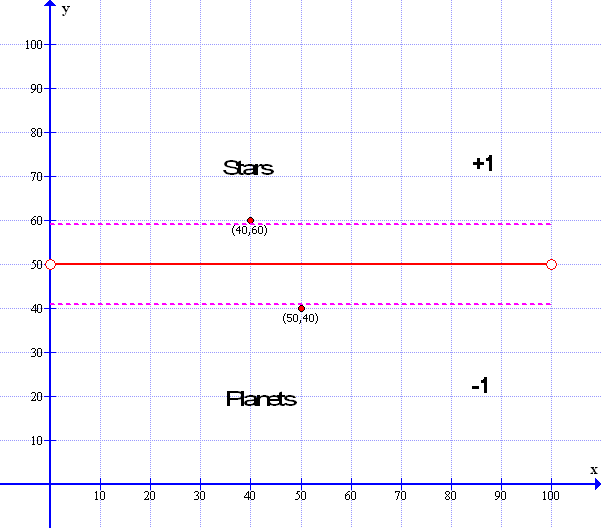
In effect if the perceptron can put a line anywhere in between the dotted areas then that line will satisfy all the conditions because a line at y=41 will make all the planets be below the line and all the stars above — the only thing we ask is that the perceptron answers all the questions correctly: all Planets labeled as -1 are below the line – and all stars labeled as +1 are above the line: To get the percepton to be more accurate we simply need to add more data points that, in itself, will get the perceptron to get much closer to the mid point line. This is why good data is important – good or sufficient data improves the result of the accuracy of our learning process.
Finally – once the Percepron has finished its learning process and has closely matched it’s guessed line with the real line we can then input a data point – Either a star or a planet – Then we can ask the perceptron a question – is this a star or is this a planet? The perceptron can then answer the question by relating that data point around it’s guessed line and if the data point comes out as +1 it is a Star otherwise it will be a Planet….And we are all deliriously happy…
A real Life example of a Perceptron in Action
So before we get into the real details of the workings – let us look at the above example running in real time, then I can use this example to illustrate the Math:- So to get it all up and running click your mouse on the panel below or, if you are on a ‘Smart’ phone, tap your screen on the panel below and it will all run for you. Stunning!
So what is happening here? The program draws our centre line in White and then fills the screen with random circles – This is our data – the Stars and Planets as in our previous example. It also allocates a small non-zero weight to the ‘Guess line’ and then draws that line in Red. All the Planets below the ‘ Guess line’ are drawn in Green and the Stars are Red It then goes through its learning algorithm by trying to find the White line so all the stars are Red above the line and all the planets are Green. There are messages as it goes along the message that reads ‘Run Closing’ Means it is within a very small margin of error – the message ‘Run Ending’ followed by ‘Completed’ means – it is the best fit that is achievable. If the message reads ‘Epoch Completed’ This means the run has ended but the line is vacillating around a few points and will go on forever so, we have limited that time to a n adequate number of repeated cycles – traditionally called an ‘epoch’. You can extend the epoch if you wish but it will do you no good – you will just watch the line vacillate for a very long time. However even with ‘Epoch Completed’ it is still within a small and acceptable margin of error.
If you wish to see it all happen again with a different set of data and different weights then, just refresh the page… Click the mouse or tap the screen and Abracadabra – it runs .. Just like magic – GTTFOMS.
So next – we will use the same learning algorithm as above to illustrate, in the coming section: the maths that make it work ( it’s really not that bad ). Now I hope you have run the program above a few times – and, as you will see, most times that the algorithm is nice and smooth and precise – other times it jumps around like a cat on a hot tin roof – now this algorithm is simple but is, probably, just as sophisticated as most in current usage – so if your bank suddenly cuts off your credit without any notice – it may not be anything you have done yourself – it might just an algorithm that has gone psycho belly up – in other words – quite normal – so, at least, in seeing what you have seen, you will, hopefully not feel so bad –
Anyway, now you can look at how all this works by clicking onto the menu tab above Perceptron 2 – the Math. Don’t worry there is only one formula to look at -. Here you will find, not only, the explanation of the program but, the program itself:- One you can mess around with – explore and play on you own computer browser. Yes, it will work on all computers – even them ‘Smart’ phones. So, for the next enthralling episode of the Perceptron you can just Click Here.
Acknowledgments:
- P5JS Code based on text “Artificial Intelligence”, George Luger
- Original coding by Daniel Shiffman -The Nature of Code – http://natureofcode.com
- Additional coding by In Variant B – http://lizziegray.net
- Graph images compiled by ‘Graph’ courtesy of Ivan Johansen
- All other graphicx by Lizzie Gray.